AP E&M Chapter 13 Analysis of Circuits
Published:
Current
Current (电流) is defined as the rate of charge flow per unit time through some surface.
\[\boxed{ I = \frac {dQ} {dt} }\]The unit of current is amp (安培). $1 \ \ce{A} = \frac {1 \ \ce{C}} {1 \ \ce{s}}$.
Resistance
The resistance (电阻) of a resistor (电阻器) is defined as the ratio of the potential difference across it to the current through it.
\[\boxed{ R = \frac V I }\]The unit of resistance is ohm (欧姆). $1 \ \Omega = \frac {1 \ \ce{V}} {1 \ \ce{A}}$.
Ohm’s law (欧姆定律) is an experimental observation, which states that the ratio $R$ is a constant.
Combinations of Resistors
In Series
Resistors in series share the same current.
\[R = \frac V I = \frac {\sum V_i} I = \sum R_i\] \[\boxed{ R_{\text{equivalent}} = \sum R_i }\]In Parallel
Resistors in parallel have the same voltage between the two sides.
\[R = \frac V I = \frac V {\sum I_i} = \frac 1 {\sum \frac 1 {R_i}}\] \[\boxed{ R_{\text{equivalent}} = \frac 1 {\sum \frac 1 {R_i}} }\]Power Dissipated Across Resistors
\[\begin{aligned} P &= \frac {dW} {dt} \\ &= \frac {\Delta V dq} {dt} \\ &= \Delta V \times I \\ \end{aligned}\]Therefore, the power dissipated across resistors is
\[\boxed{ P = VI }\]Voltmeters and Ammeters
Voltmeters (电压表) are devices that measure voltage, and ammeters (电流表) are devices that measure current.
Kirchhoff’s Laws
- The node rule (KCL, 基尔霍夫电流定律): At any intersection of wires, the total current entering the intersection must equal the total current leaving the intersection.
- The loop rule (KVL, 基尔霍夫电压定律): The sum of the potential differences around any closed loop must be zero.
Example 13.5
For the circuit in Figure 13.5, calculate the magnitude and direction of current through each wire.
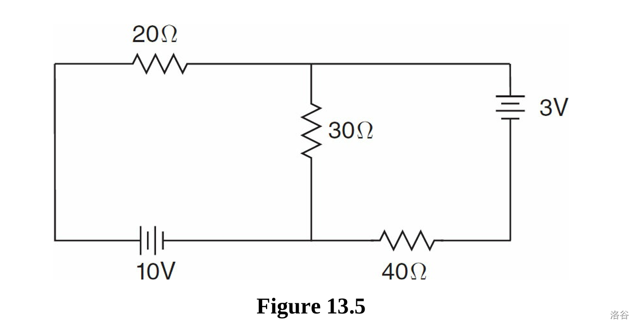
See this new figure:
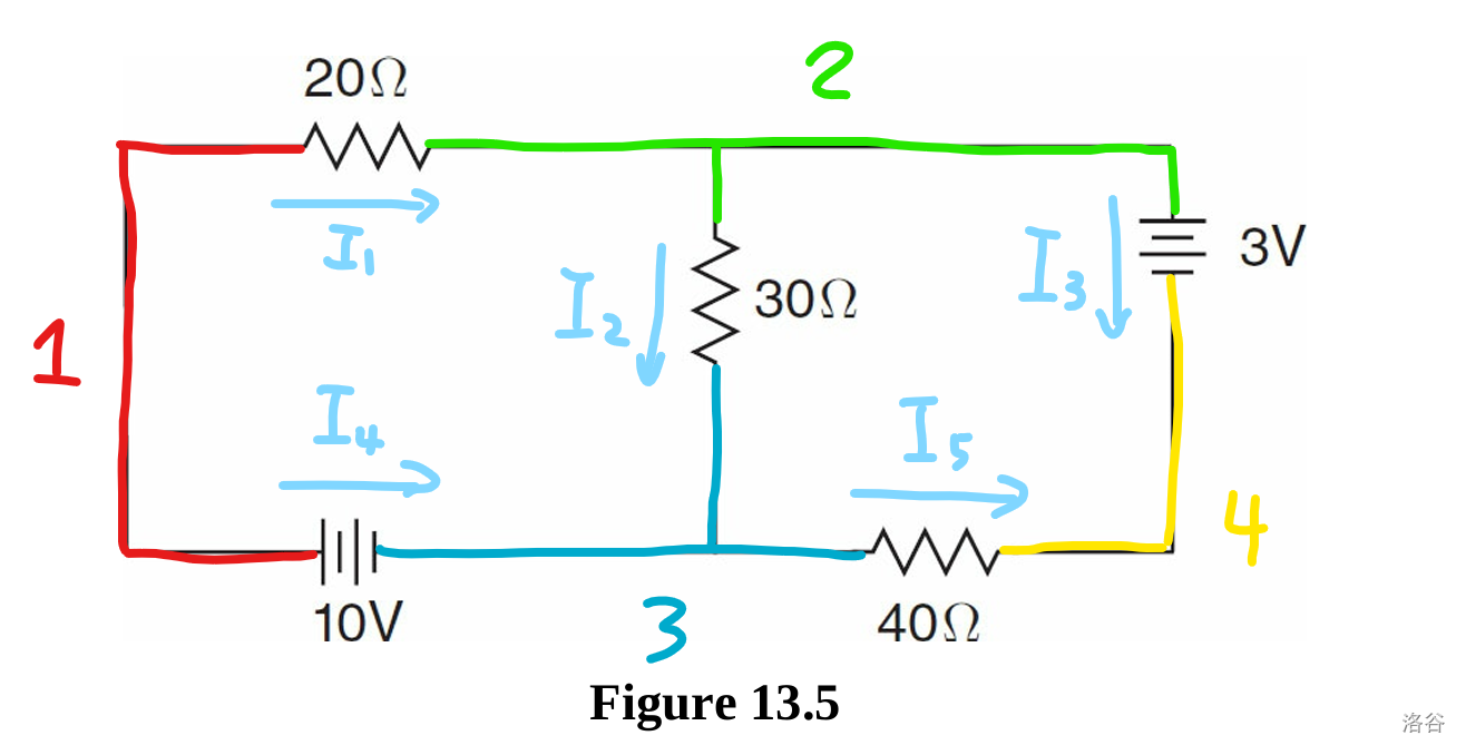
We have $4$ nodes labeled by different colors, and we have $5$ edges. We label the direction of current on each edge randomly.
\[\begin{cases} - I_1 - I_4 = 0 & \text{Node 1} \\ I_1 - I_2 - I_3 = 0 & \text{Node 2} \\ I_2 + I_4 - I_5 = 0 & \text{Node 3} \\ 20\Omega I_1 + 30\Omega I_2 + 10V = 0 \\ 30\Omega I_2 + 40\Omega I_5 + 3V = 0 \\ \end{cases}\]For a circuit with $n$ nodes and $m$ edges, we create $n-1$ equations using the node rule and $m-n+1$ equations using the loop rule.
- The $n-1$ KCL equations can be chosen arbitrarily.
- The method of choosing $m-n+1$ KVL equations is more complex.
💡 How to find proper KVL equations?
- Find a spanning tree of the circuit.
- For each edge not in the spanning tree, find a cycle containing only this edge and edges in the tree. This cycle is called a fundamental cycle with respect to the spanning tree.
- Create a KVL equation for each of the fundamental cycles.
This principle is guaranteed by some results in linear algebra, which will be discussed in future blogs.
Solving the linear equation system, we derive
\[\begin{cases} I_2 = - \frac {23} {130} \ce{A} \\ I_4 = - I_1 = \frac {61} {260} \ce{A} \\ I_5 = - I_3 = \frac {3} {52} \ce{A} \\ \end{cases}\]Don’t be surprised that we get negative answers for currents. In fact, it simply means that we chose the wrong direction for the current.
RC Circuits

Charging a Capacitor
When the switch is connected to a, the circuit is charging the capacitor.
We can write the equation of Ohm’s Law ($V = IR$) for this circuit:
\[V - \frac Q C = \frac {dQ} {dt} R\]Solving the differential equation with initial condition $Q(0) = 0$, we derive
\[\boxed{ Q(t) = Q_{\text{final}} (1 - e^{- \frac t {RC}}) }\]where $Q_{\text{final}} = Q(\infty) = CV$.
Take the derivative of $Q$ with respect to time, we can calculate the current:
\[\boxed{ I(t) = I_0 e^{- \frac t {RC}} }\]where $I_0 = \frac V R$ is the initial current.
Discharging a Capacitor
When the switch is connected to b, the circuit is discharging the capacitor.
By the same process we can calculate the charge on the capacitor and the current through the capacitor:
\[\boxed{ Q(t) = Q_0 e^{- \frac t {RC}} }\] \[\boxed{ I(t) = I_0 e^{- \frac t {RC}} }\]where $Q_0 = Q(0)$ is the initial charge and $I_0 = \frac Q {RC}$ is the initial current.
Time Constant for RC Circuits
Note that $e^{- \frac t {RC}}$ appears in all those equations. Therefore, in order to simplify these equations, we define the time constant $\tau$ as:
\[\boxed{ \tau = RC }\]and then these exponential terms become to $e^{- \frac t \tau}$.